Aside: Animate a NN

Libraries

Code

library(tidyverse)
library(nnet)
library(ggthemes)
library(gganimate)
library(av)

As usual we’ll want tidyverse(Wickham 2023). The main function for the NN we will be using is in nnet(Ripley 2025). We’ll be doing some animations and want ggthemes(Arnold 2025), gganimate(Pedersen and Robinson 2025), and av(Ooms 2025).

The Data

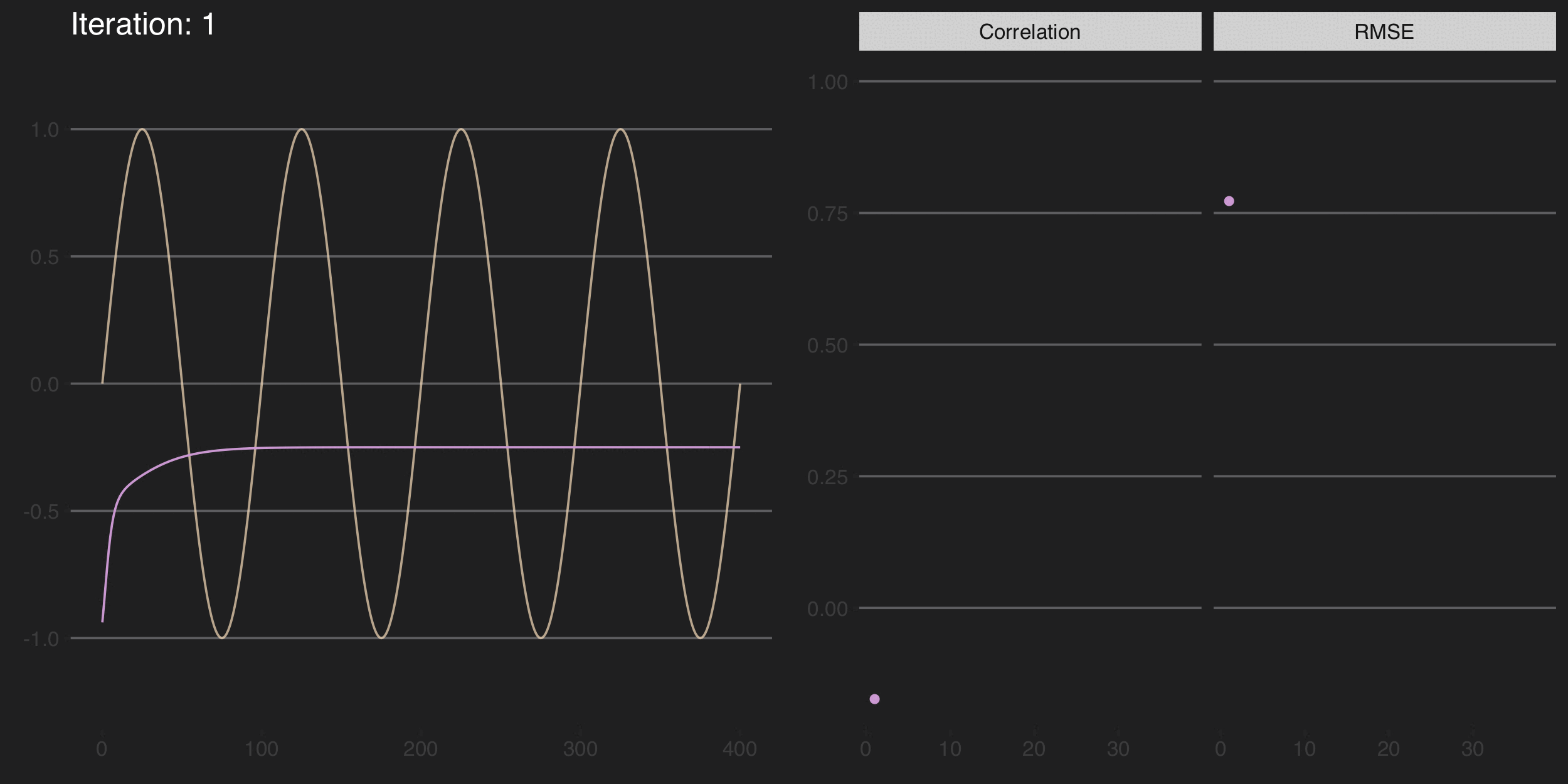
Here is a quick demo of how a neural network successively iterates to improve fit. We will create a simple sine wave and then ask a neural net to try to predict it. We will animate that process by saving the prediction at each iteration.

Here is the function and the data to fit.

Code

n <- 400
dat <- tibble(x = seq(0,n),
              y = sin(2 * pi / 100 * seq(0,n)))
dat %>% ggplot(mapping = aes(x=x,y=y)) +
  geom_line(color="#fbe4c6", alpha=0.7) +
  labs(x=element_blank(),y=element_blank()) + 
  theme_hc(style = 'darkunica') +
  theme(legend.position = "none",
        text=element_text(size=12))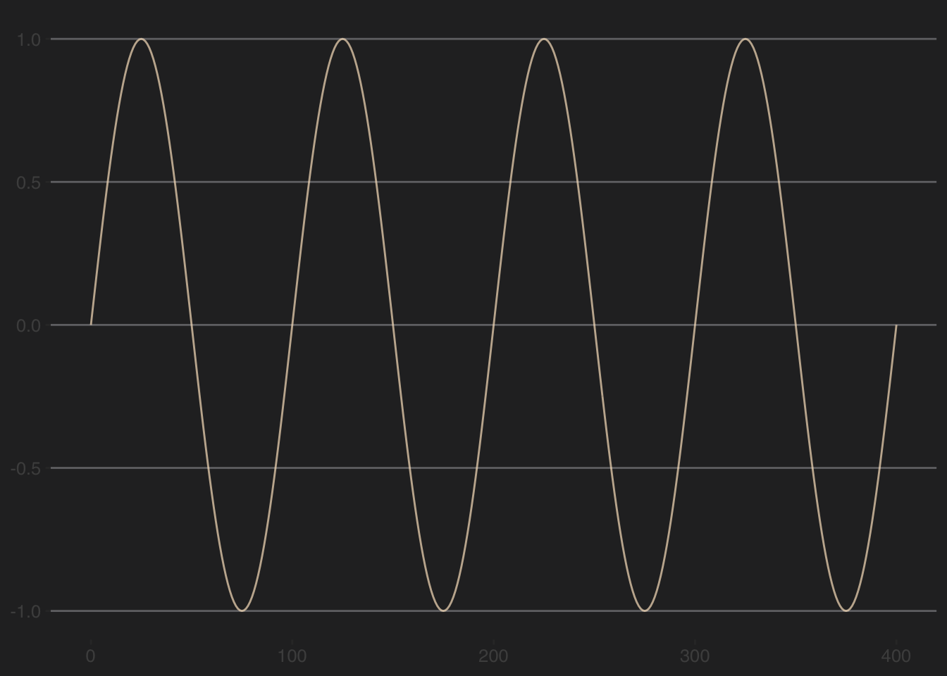

Predicting

We will use a single-hidden-layer neural network to fit to the data. We do some cumbersome looping in order to save the predictions from each iteration. If the fit is really really good (r > 0.999) the loop will quit. With this simple sine function, that criteria is usually met.

Code

nIter <- 100
fits <- as_tibble(matrix(0,nrow=length(dat$x),ncol=nIter))
gof <- tibble(Iter = 1:nIter, Correlation = numeric(nIter), RMSE = numeric(nIter)) 
for(i in 1:nIter){
  if(i==1) {
    # because i=1 we start without weights
    nn <- nnet(dat$x, dat$y, size=10, maxit=i-1, linout=TRUE, trace = FALSE)
  }
  else {
    # use prior weights to start the nnet once they exist (i>1)
    nn <- nnet(dat$x, dat$y, size=10, maxit=i-1, linout=TRUE, trace = FALSE, Wts = nn$wts)
  }
  yhat <- predict(nn)[,1]
  fits[,i] <- yhat
  gof$Correlation[i] <- cor(dat$y,yhat)
  gof$RMSE[i] <- sqrt(mean((dat$y-yhat)^2))
  # if fits are ~perfect, stop
  if(gof$Correlation[i] > 0.9995) { break }
}
# trim fits if loop stopped early
fits <- fits[,1:i]
fits2 <- as_tibble(cbind(dat$x,fits)) 
names(fits2)[1] <- "x"
names(fits2)[-1] <- formatC(1:i,digits = 1,flag=0)
gof <- gof[1:i,]
tail(gof)

# A tibble: 6 × 3
   Iter Correlation   RMSE
  <int>       <dbl>  <dbl>
1    33       0.979 0.146 
2    34       0.980 0.142 
3    35       0.983 0.130 
4    36       0.993 0.0822
5    37       0.999 0.0338
6    38       1.000 0.0195

Above, the loop reached 38 iterations before the fit was essentially perfect. Let’s see all the predictions.

Code

fits2 <- fits2 %>% 
  pivot_longer(cols=-1,names_to = "IterChar", values_to = "yhat") %>%
  mutate(Iter = as.numeric(IterChar))

p1 <- ggplot(fits2,aes(x=x,y=yhat,color=IterChar)) +
  # original data
  geom_line(data=dat,aes(x=x,y=y),inherit.aes = FALSE, 
            color="#fbe4c6", alpha=0.7) +
  # nn fits
  geom_line() + 
  scale_color_manual(values=PNWColors::pnw_palette("Spring",i)) +
  labs(x=NULL,y=NULL) +
  theme_hc(style = 'darkunica') +
  theme(legend.position = "none",
        text=element_text(size=12))
p1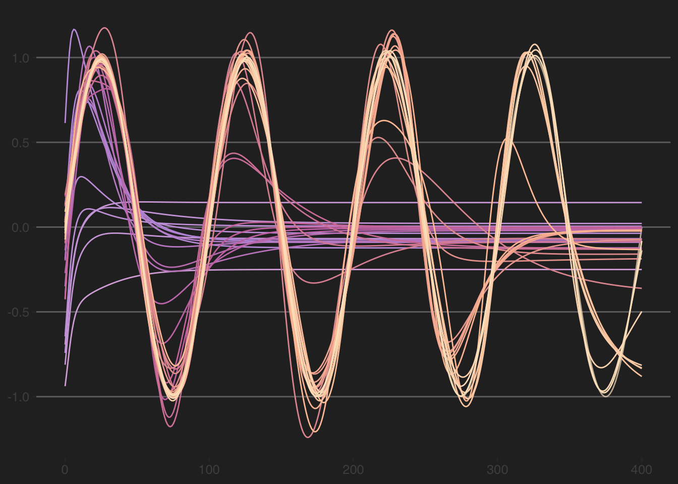

And the evolution of the RMSE and the correlation (r).

Code

gof2 <- gof %>% pivot_longer(cols = -1)    
p2 <- ggplot(gof2,aes(x=Iter,y=value,color=Iter)) +
  geom_point() + geom_line() +
  scale_color_gradientn(colors=PNWColors::pnw_palette("Spring",i)) +
  labs(x="Iteration",y=NULL) +
  facet_wrap(~name) +
  theme_hc(style = 'darkunica') +
  theme(legend.position = "none",
        text=element_text(size=12))
p2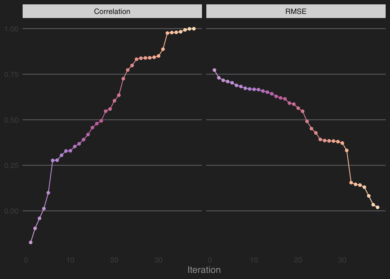

Animate

Below is a combo of the fits and the skill in a GIF. Note that combining the two plots to have it all work side by side is a little more complicated than I’d like it to be and we have to use the magick library. See here. I hid the code because it’s yucky and confusing. But it’s on the repo in the Rmd file if you want to see it.